파이토치를 사용해서 멀티 퍼셉트론 구현하기 !
iris 데이터를 사용해서 붓꽃의 종류를 분류해보자 ~
PyTorch
PyTorch는 Python을 위한 오픈소스 머신 러닝 라이브러리 !
GPU사용이 가능하기 때문에 속도가 상당히 빠르다
파이토치를 사용하는 이유는
1. 파이썬과 유사해서 코드를 이해하기 쉽다
2. 설정과 실행이 매우 쉽다
3. 딥러닝을 배우기 쉽다
4. 연구에도 많이 사용된다
등 ~
IRIS 데이터셋
붓꽃에 대한 데이터 !
꽃받침의 길이, 너비와 꽃잎의 길이, 너비에 대한 4차원 데이터이다
1. PyTorch 설치
일단 내 개발환경은 맥이기 때문에 mac 기준으로 진행
Anaconda | Anaconda Distribution
Anaconda's open-source Distribution is the easiest way to perform Python/R data science and machine learning on a single machine.
www.anaconda.com
아나콘다 설치를 해줍니다
맥은 anaconda power shell이 따로 없고 cmd창이 (base)가 붙으면 활성화된 것 !

그리고 파이썬과 아나콘다의 버전을 확인해줍니다
다음으로는 conda로 파이토치를 설치 !
PyTorch
An open source machine learning framework that accelerates the path from research prototyping to production deployment.
pytorch.org
conda install pytorch torchvision torchaudio -c pytorch시킨대로.. 명령 실행 !
제대로 설치됐는지 확인을 해보면..!
샘플 PyTorch 코드를 실행해서 임의로 초기화된 텐서를 구성 ~
2. 모델에 대한 데이터 설정
데이터셋 다운
Fisher의 붓꽃 데이터 세트에서 모델을 학습 !
이 데이터셋에는 부채붓꽃(Iris setosa), 버시컬러 붓꽃(Iris versicolor) 및 버지니카 붓꽃(Iris virginica)의 세 가지 붓꽃 종 각각에 대한 50개의 레코드가 포함되어 있다고 함
우선 IRIS 데이터를 엑셀 파일로 저장
GitHub - microsoft/Windows-Machine-Learning: Samples and Tools for Windows ML.
Samples and Tools for Windows ML. Contribute to microsoft/Windows-Machine-Learning development by creating an account on GitHub.
github.com
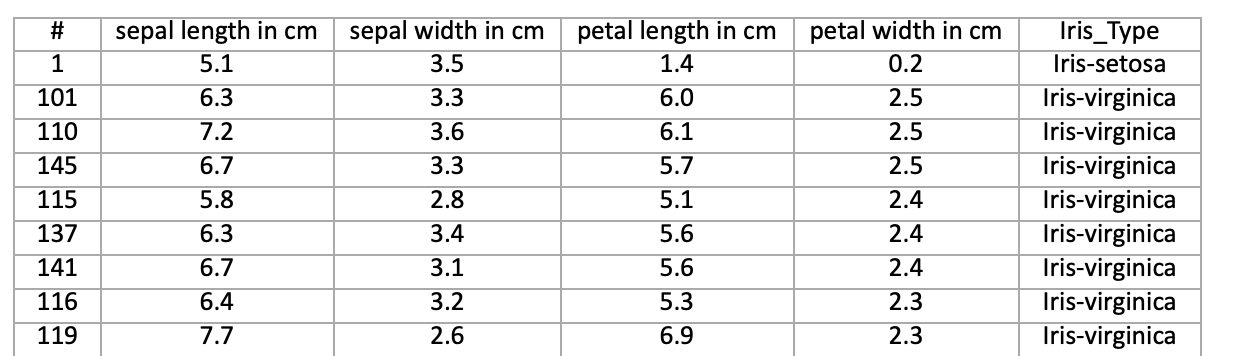
붓꽃의 네 가지 특징과 종류가 있음 !
패키지 엑세스
import torch
import pandas as pd
import torch.nn as nn
from torch.utils.data import random_split, DataLoader, TensorDataset
import torch.nn.functional as F
import numpy as np
import torch.optim as optim
from torch.optim import Adam
파이썬 데이터 분석에 사용되는 pandas 패키지도 이용해 torch.nn 패키지(데이터 및 신경망 구축을 위한 모듈과 확장 가능한 클래스가 포함) 로드
데이터셋 로드
데이터 로드 -> 클래스 수 확인
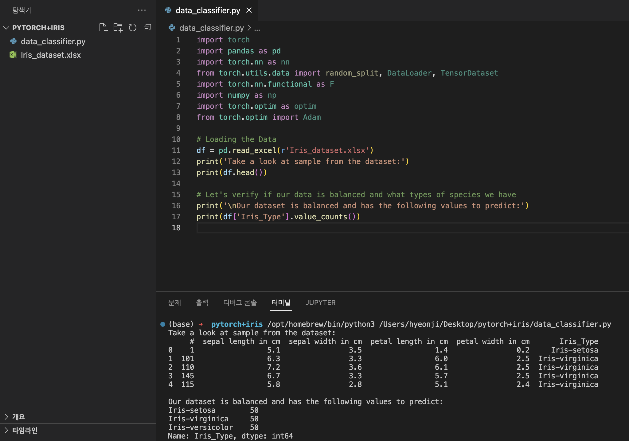
# Loading the Data
df = pd.read_excel(r'C:…\Iris_dataset.xlsx')
print('Take a look at sample from the dataset:')
print(df.head())

# Let's verify if our data is balanced and what types of species we have
print('\nOur dataset is balanced and has the following values to predict:')
print(df['Iris_Type'].value_counts())
여기서 나는 Iris_dataset.xlsx 파일의 경로를 내 환경에 맞게 수정해주었다
쨔잔 ~
데이터셋을 사용하고 모델을 학습하기 위해 입력 및 출력을 정의해준다
입력에는 150개의 특징이 포함되어 있고, 출력은 붓꽃 종류 열이다
사용할 신경망에는 숫자 변수가 필요하기 때문에 출력 변수를 숫자 형식으로 변환한다
숫자 형식으로 출력 표시 & 데이터셋에 새 열 추가
# Convert Iris species into numeric types: Iris-setosa=0, Iris-versicolor=1, Iris-virginica=2.
labels = {'Iris-setosa':0, 'Iris-versicolor':1, 'Iris-virginica':2}
df['IrisType_num'] = df['Iris_Type']   # Create a new column "IrisType_num"
df.IrisType_num = [labels[item] for item in df.IrisType_num]  # Convert the values to numeric ones

# Define input and output datasets
input = df.iloc[:, 1:-2]            # We drop the first column and the two last ones.
print('\nInput values are:')
print(input.head())
output = df.loc[:, 'IrisType_num']   # Output Y is the last column
print('\nThe output value is:')
print(output.head())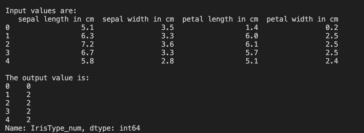
여기서 모델을 학습하기 위해선 모델 입력 및 출력 형식으로 텐서로 변환해준다
텐서로 변환
# Convert Input and Output data to Tensors and create a TensorDataset
input = torch.Tensor(input.to_numpy())      # Create tensor of type torch.float32
print('\nInput format: ', input.shape, input.dtype)     # Input format: torch.Size([150, 4]) torch.float32
output = torch.tensor(output.to_numpy())        # Create tensor type torch.int64
print('Output format: ', output.shape, output.dtype)  # Output format: torch.Size([150]) torch.int64
data = TensorDataset(input, output)    # Create a torch.utils.data.TensorDataset object for further data manipulation
입력 값은 150개이고, 이 중 60%는 모델 학습 데이터, 유효성 검사(val) 20%, 테스트(test) 30%로 나눠준다
데이터 분할
# Split to Train, Validate and Test sets using random_split
train_batch_size = 10
number_rows = len(input)    # The size of our dataset or the number of rows in excel table.
test_split = int(number_rows*0.3)
validate_split = int(number_rows*0.2)
train_split = number_rows - test_split - validate_split
train_set, validate_set, test_set = random_split(
    data, [train_split, validate_split, test_split])

# Create Dataloader to read the data within batch sizes and put into memory.
train_loader = DataLoader(train_set, batch_size = train_batch_size, shuffle = True)
validate_loader = DataLoader(validate_set, batch_size = 1)
test_loader = DataLoader(test_set, batch_size = 1)
3. PyTorch 모델 학습
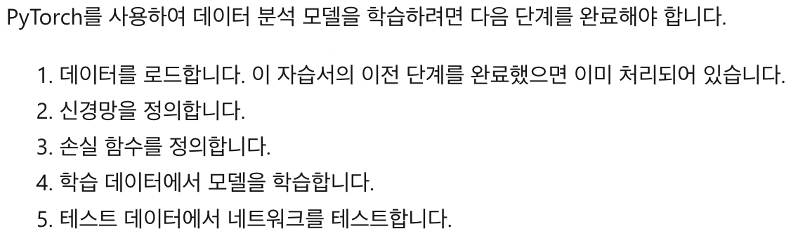
신경망 정의
여기서는 세 개의 선형 계층을 사용해 기본 신경망 모델을 빌드 !
Linear -> ReLU -> Linear -> ReLU -> Linear
Linear : 들어오는 데이터에 선형 변환 적용, 클래스 수에 해당하는 입력, 출력 수를 지정해야 함
ReLU : 들어오는 모든 기능을 0 이상으로 정의하는 활성화 함수, 0보다 작은 숫자는 0으로 변경되고 나머지는 유지
-> 두 개의 계층에 활성화 계층을 적용하고 마지막 선형 계층에서는 활성화를 적용하지 않음
모델의 매개 변수 + 신경망 정의
모델의 매개 변수는 목표와 학습 데이터에 따라 달라진다
입력 크기는 모델을 제공하는 기능 수에 따라 달라짐 (iris 데이터의 경우 4)
iris 데이터의 출력 크기는 3 (세 가지 종류의 붓꽃)
3개의 선형 계층((4,24) -> (24,24) -> (24,3))이 있는 네트워크에는 744개의 가중치(96+576+72)가 있음
lr(학습 속도)은 손실 그레이디언트와 관련하여 네트워크의 가중치를 조정하는 정도에 대한 제어를 설정
이 값이 낮을수록 학습 속도가 느려짐 -> 여기서는 0.01로 설정
학습 중 모든 계층을 통해 입력 처리 -> 손실 계산 -> 예측 레이블과 올바른 레이블의 다른 정보 파악 -> 그레이디언트를 네트워크에 재전파 -> 계층 가중치 업데이트 => 방대한 입력 데이터셋을 반복해 가중치 설정하는 방법을 학습
정방향 함수는 손실 함수의 값을 계산 + 역방향 함수는 학습 가능한 매개 변수의 그레이디언트 계산
pytorch를 사용해 신경망을 만드는 경우 정방향 함수만 정의 (역방향 함수는 자동으로 정의됨)
모델의 매개 변수와 신경망을 정의해줍니다
# Define model parameters
input_size = list(input.shape)[1]   # = 4. The input depends on how many features we initially feed the model. In our case, there are 4 features for every predict value
learning_rate = 0.01
output_size = len(labels)           # The output is prediction results for three types of Irises.


# Define neural network
class Network(nn.Module):
   def __init__(self, input_size, output_size):
       super(Network, self).__init__()

       self.layer1 = nn.Linear(input_size, 24)
       self.layer2 = nn.Linear(24, 24)
       self.layer3 = nn.Linear(24, output_size)


   def forward(self, x):
       x1 = F.relu(self.layer1(x))
       x2 = F.relu(self.layer2(x1))
       x3 = self.layer3(x2)
       return x3

# Instantiate the model
model = Network(input_size, output_size)
실행 디바이스 정의
PC에서 사용 가능한 실행 디바이스를 기준으로 실행 디바이스를 정의
디바이스는 Nvidia GPU가 컴퓨터에 있으면 Nvidia GPU가 되고, 없으면 CPU로 설정됨
# Define your execution device
device = torch.device("cuda:0" if torch.cuda.is_available() else "cpu")
print("The model will be running on", device, "device\n")
model.to(device)    # Convert model parameters and buffers to CPU or Cuda
모델 저장
# Function to save the model
def saveModel():
    path = "./NetModel.pth"
    torch.save(model.state_dict(), path)
손실 함수 정의
손실 함수는 출력이 대상과 다른 정도를 예측하는 값을 계산
주요 목표는 신경망의 역방향 전파를 통해 가중치 벡터 값을 변경하여 손실 함수의 값을 줄이는 것 !
손실 값은 모델 정확도와 다름! 손실 함수는 학습 세트에서 최적화를 반복할 때마다 모델이 얼마나 잘 작동하는지 나타냄
(모델의 정확도는 테스트 데이터에서 계산되며 정확한 예측의 백분율)
여기서는 분류에 최적화된 기존 함수를 사용, Classification Cross-Entropy 손실 함수와 Adam 최적화 프로그램을 사용
최적화 프로그램에서 lr(학습 속도)은 손실 그레이디언트와 관련하여 네트워크의 가중치를 조정하는 정도에 대한 제어를 설정합니다. 여기서는 0.001로 설정
# Define the loss function with Classification Cross-Entropy loss and an optimizer with Adam optimizer
loss_fn = nn.CrossEntropyLoss()
optimizer = Adam(model.parameters(), lr=0.001, weight_decay=0.0001)
모델 학습
학습 세트에 걸친 모든 Epoch 또는 모든 전체 반복에 대해 학습 손실, 유효성 검사 손실 및 모델의 정확도를 표시
가장 높은 정확도로 모델을 저장하고 10번의 Epoch 후에 프로그램이 최종 정확도를 표시
# Training Function
def train(num_epochs):
    best_accuracy = 0.0

    print("Begin training...")
    for epoch in range(1, num_epochs+1):
        running_train_loss = 0.0
        running_accuracy = 0.0
        running_vall_loss = 0.0
        total = 0

        # Training Loop
        for data in train_loader:
        #for data in enumerate(train_loader, 0):
            inputs, outputs = data  # get the input and real species as outputs; data is a list of [inputs, outputs]
            optimizer.zero_grad()   # zero the parameter gradients
            predicted_outputs = model(inputs)   # predict output from the model
            train_loss = loss_fn(predicted_outputs, outputs)   # calculate loss for the predicted output
            train_loss.backward()   # backpropagate the loss
            optimizer.step()        # adjust parameters based on the calculated gradients
            running_train_loss +=train_loss.item()  # track the loss value

        # Calculate training loss value
        train_loss_value = running_train_loss/len(train_loader)

        # Validation Loop
        with torch.no_grad():
            model.eval()
            for data in validate_loader:
               inputs, outputs = data
               predicted_outputs = model(inputs)
               val_loss = loss_fn(predicted_outputs, outputs)

               # The label with the highest value will be our prediction
               _, predicted = torch.max(predicted_outputs, 1)
               running_vall_loss += val_loss.item()
               total += outputs.size(0)
               running_accuracy += (predicted == outputs).sum().item()

        # Calculate validation loss value
        val_loss_value = running_vall_loss/len(validate_loader)

        # Calculate accuracy as the number of correct predictions in the validation batch divided by the total number of predictions done.
        accuracy = (100 * running_accuracy / total)

        # Save the model if the accuracy is the best
        if accuracy > best_accuracy:
            saveModel()
            best_accuracy = accuracy

        # Print the statistics of the epoch
        print('Completed training batch', epoch, 'Training Loss is: %.4f' %train_loss_value, 'Validation Loss is: %.4f' %val_loss_value, 'Accuracy is %d %%' % (accuracy))
테스트 데이터로 모델 테스트
두 개의 테스트 함수를 추가
첫 번째는 이전 파트에서 저장한 모델을 테스트
45개 항목의 테스트 데이터 세트로 모델을 테스트하고 모델의 정확도를 출력
두 번째는 세 가지 붓꽃 종 중에서 각 종을 성공적으로 분류하는 확률을 예측하는 모델의 신뢰도를 테스트하는 선택적 함수
# Function to test the model
def test():
    # Load the model that we saved at the end of the training loop
    model = Network(input_size, output_size)
    path = "NetModel.pth"
    model.load_state_dict(torch.load(path))

    running_accuracy = 0
    total = 0

    with torch.no_grad():
        for data in test_loader:
            inputs, outputs = data
            outputs = outputs.to(torch.float32)
            predicted_outputs = model(inputs)
            _, predicted = torch.max(predicted_outputs, 1)
            total += outputs.size(0)
            running_accuracy += (predicted == outputs).sum().item()

        print('Accuracy of the model based on the test set of', test_split ,'inputs is: %d %%' % (100 * running_accuracy / total))


# Optional: Function to test which species were easier to predict
def test_species():
    # Load the model that we saved at the end of the training loop
    model = Network(input_size, output_size)
    path = "NetModel.pth"
    model.load_state_dict(torch.load(path))

    labels_length = len(labels) # how many labels of Irises we have. = 3 in our database.
    labels_correct = list(0. for i in range(labels_length)) # list to calculate correct labels [how many correct setosa, how many correct versicolor, how many correct virginica]
    labels_total = list(0. for i in range(labels_length))   # list to keep the total # of labels per type [total setosa, total versicolor, total virginica]

    with torch.no_grad():
        for data in test_loader:
            inputs, outputs = data
            predicted_outputs = model(inputs)
            _, predicted = torch.max(predicted_outputs, 1)

            label_correct_running = (predicted == outputs).squeeze()
            label = outputs[0]
            if label_correct_running.item():
                labels_correct[label] += 1
            labels_total[label] += 1

    label_list = list(labels.keys())
    for i in range(output_size):
        print('Accuracy to predict %5s : %2d %%' % (label_list[i], 100 * labels_correct[i] / labels_total[i]))
마지막으로, 주 코드를 추가
모델 학습이 시작, 모델 저장, 결과가 화면에 표시
학습 세트에 대해 두 번의 반복([num_epochs = 25])만 실행 -> 학습 프로세스가 너무 오래 걸리지 않음
if __name__ == "__main__":
    num_epochs = 10
    train(num_epochs)
    print('Finished Training\n')
    test()
    test_species()
결과..!
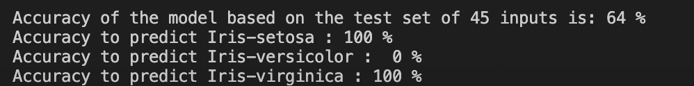
음.. 저는 왜 이래요....................
지쳤도다....
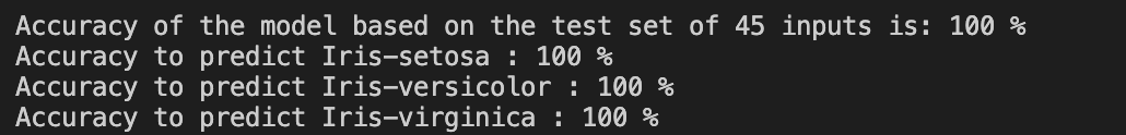
에.. 내가 참고한 글에서는 엑셀 파일에서 #가 오름차순으로 돼있길래 정렬하고 다시 돌렸더니..
근데 여러 번 돌리면 싹싹 변해 아주..
어차피 셔플하는데 이게 무슨 소용이람
아래는 내가 참고한 글
PyTorch 및 Windows ML을 사용한 데이터 분석
PyTorch를 사용하여 ML 데이터 분석 모델을 만들고 ONNX로 내보내고 로컬 앱에 배포하는 단계 알아보기
learn.microsoft.com
감사합니다... 덕분에 엉덩이 붙이고 글 읽고 따라하기만 했는데 아이리스 분류 모델을 만들기는 했어요..
두 번째 종류 정확도는 0%이지만...
아래 글은 뭔가 도움이 될 것 같아서 가져와봤다 나중에 이걸로 해봐야지
입문자를 위한 머신러닝 분류 튜토리얼 - IRIS 분류
개요 사이킷런(scikit-learn)은 파이썬 머신러닝 라이브러리이다. 파이썬에서 나오는 최신 알고리즘들도 이제는 사이킷런에 통합하는 형태로 취하고 있다. 구글 코랩은 기본적으로 사이킷런까지
dschloe.github.io
Classifying the Iris Data Set with PyTorch
In this short article we will have a look on how to use PyTorch with the Iris data set. We will create and train a neural network with Linear layers and we will employ a Softmax activation function and the Adam optimizer.
janakiev.com
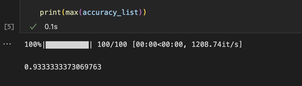
사실 두번째 글도 따라서 해봤는데 (제대로 공부하진 않았도다)

's t u d y . . 🍧 > AI 앤 ML 앤 DL' 카테고리의 다른 글
| [ML 이론] 기계학습이란 (0) | 2023.05.01 |
|---|---|
| [NLP | BERT & SBERT] Cross-Encoder와 Bi-Encoder (0) | 2023.04.27 |
| [Transfer Learning] 전이학습 개념 (1) | 2022.10.08 |
| [YOLOv5] 학습된 모델로 이미지 test 후 한 파일에 저장하기 (0) | 2022.10.08 |
| [YOLOv5] YOLOv5 사용법 (1) | 2022.10.07 |